Model Building Process
Unveiling the Secrets of Superhero Power: A Data-driven Approach
Have you ever been curious about what makes a superhero truly powerful? Is it their intelligence, physical strength, or probably the combination of the factors that determines their success? In this analysis, we delve into a data-driven approach to uncover the key traits that determine superhero power, using statistical and machine learning techniques to identify patterns and interactions.
library(tidyverse)
library(modelr)
library(mice)
library(mgcv)
library(randomForest)
library(readr)
library(dplyr)
library(patchwork)
library(car)
set.seed(1)
Variables Selection
Methods
We first do univariate analyses to predict the power by intelligence, strength, speed, durability, combat, height, weight, gender, and alignment respectively.
superheros <- read_csv("./data/superheroes.csv")

superheros_clean1 <- superheros %>%
  filter(complete.cases(intelligence, strength, speed, durability, combat, height_cm, weight_kg, gender, alignment, power))

superheros_clean1$gender <- as.factor(superheros_clean1$gender)
superheros_clean1$alignment <- as.factor(superheros_clean1$alignment)


# we first do univariate analysis to find variables that significantly associate with the power with p value < 0.05
univariate_analysis = function(var, var_name){
  model = summary(lm(power ~ var, data = superheros_clean1))

  p_value = model$coefficients[2, 4]

  return(data.frame(variable = var_name, p_value = p_value))
}

results = rbind(
  univariate_analysis(superheros_clean1$intelligence, "Intelligence"),
  univariate_analysis(superheros_clean1$strength, "Strength"),
  univariate_analysis(superheros_clean1$speed, "Speed"),
  univariate_analysis(superheros_clean1$durability, "Durability"),
  univariate_analysis(superheros_clean1$combat, "Combat"),
  univariate_analysis(superheros_clean1$height_cm, "Height"),
  univariate_analysis(superheros_clean1$weight_kg, "Weight"),
  univariate_analysis(superheros_clean1$gender, "Gender"),
  univariate_analysis(superheros_clean1$alignment, "Alignment")
)

results$p_value <- round(results$p_value, 4)

library(knitr)
kable(results, col.names = c("Variable", "P-Value"), digits = 4, align = "c")| Variable | P-Value |
|---|---|
| Intelligence | 0.0000 |
| Strength | 0.0000 |
| Speed | 0.0000 |
| Durability | 0.0000 |
| Combat | 0.0615 |
| Height | 0.1282 |
| Weight | 0.0394 |
| Gender | 0.3960 |
| Alignment | 0.6718 |
Based on the results, we found intelligence,
strength, speed, durability,
weight are significantly associated with the power with
p-value < 0.05.
Building Linear Regression Model
We build a linear regression model to predict the power of superheros based on the four variables we identified.
sig_model = lm(power ~ intelligence + strength + speed + durability + weight_kg, data = superheros_clean1)

sig_model %>%
  broom::tidy() %>%
  dplyr::select(term, estimate, p.value) %>%
knitr::kable(digits = 4)| term | estimate | p.value |
|---|---|---|
| (Intercept) | 19.6052 | 0.0001 |
| intelligence | 0.2065 | 0.0010 |
| strength | 0.1037 | 0.0491 |
| speed | 0.3254 | 0.0000 |
| durability | 0.2704 | 0.0000 |
| weight_kg | -0.0165 | 0.1917 |
# Intelligence, strength, speed, durability, speed, weight are significant predictors Based on the results, we see that 4 of the variables are
statistically significant at 0.05 significance level. The effect of
weight is not statistically significant at the 0.05 level.
Superheroes’ power is positively related to
intelligence, strength, speed,
and durability, while negatively related to
weight.
Model Selection
Performing forward, backward, and stepwise model selection
After performing forward, backward, and stepwise model selection,
only the effect of durability, speed, and
intelligence were significant, therefore, we included them
in the regression model A. Since we had identified that the effect of
strength is also significant, we included
durability, speed, intelligence,
and strength in the second linear regression model. For the
last linear regression model, all 9 variables were included.
The three models we built are:
Model A: Power ~ Intelligence, speed, durability
# After having forward/backward/stepwise model selection, durability, speed, intelligence, and strength are left in the model, and only durability, speed, intelligence are significant.

lm_modelA <- lm(power ~ intelligence + speed + durability, data = superheros_clean1) %>%
  broom::tidy() %>%
  dplyr::select(term, estimate, p.value)
Model B: Power ~ Intelligence, strength, speed, durability
lm_modelB <- lm(power ~ intelligence + strength + speed + durability, data = superheros_clean1) %>%
  broom::tidy() %>%
  dplyr::select(term, estimate, p.value)
Model C: Power ~ Intelligence, strength, speed, durability, combat, height_cm, weight_kg, alignment, gender
lm_modelC <- lm(power ~ intelligence + strength + speed + durability + combat + height_cm + weight_kg + alignment + gender, data = superheros_clean1) %>%
  broom::tidy() %>%
  dplyr::select(term, estimate, p.value)
Model Evaluation
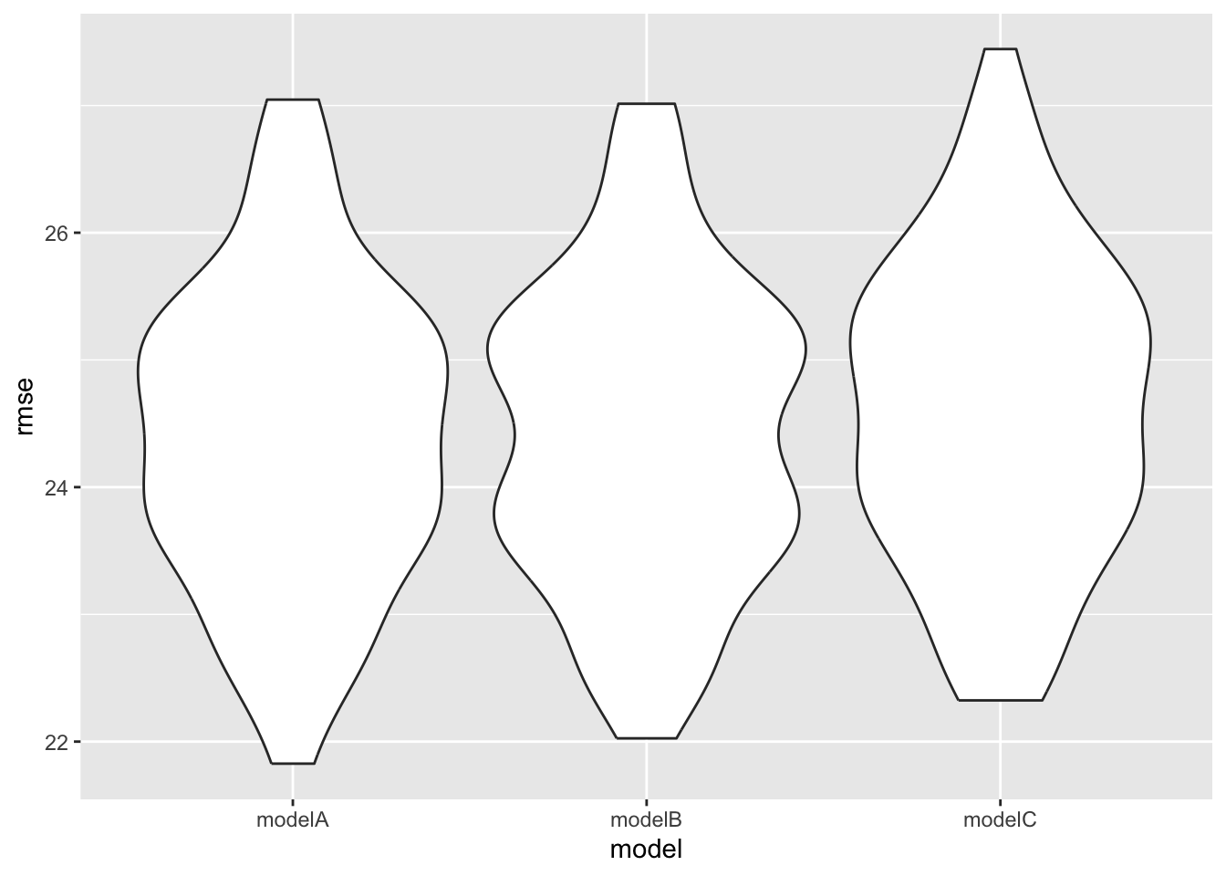
We wanted to compare the predictive performance of these 3 competing methods by using cross validation for repeating 100 times, and then comparing distribution of Root Mean Squared Error (RMSE) and of AIC of each model.
cv_df =
  crossv_mc(superheros_clean1, 100) |>
  mutate(
    train = map(train, as_tibble),
    test = map(test, as_tibble))

cv_df =
  cv_df |>
  mutate(
    lm_modelA  = map(train, \(df) lm(power ~ intelligence + speed + durability, data = df)),
    lm_modelB = map(train, \(df) lm(power ~ intelligence + strength + speed + durability, data = df)),
    lm_modelC = map(train, \(df) lm(power ~ intelligence + strength + speed + durability + combat + height_cm + weight_kg + alignment, data = df))) %>%
  mutate(
    rmse_modelA = map2_dbl(lm_modelA, test, \(mod, df) rmse(model = mod, data = df)),
    rmse_modelB = map2_dbl(lm_modelB, test, \(mod, df) rmse(model = mod, data = df)),
    rmse_modelC = map2_dbl(lm_modelC, test, \(mod, df) rmse(model = mod, data = df)))

cv_df |>
  dplyr::select(starts_with("rmse")) |>
  pivot_longer(
    everything(),
    names_to = "model",
    values_to = "rmse",
    names_prefix = "rmse_") |>
  mutate(model = fct_inorder(model)) |>
  ggplot(aes(x = model, y = rmse)) + geom_violin()
Although model A has similar RMSE distribution with model B, model B has
the relatively lowest RMSE distribution overall. Moreover, model B has
the lowest AIC value. Therefore, model B is the model has good
predictive accuracy.
Random Forest to Verify Predictors
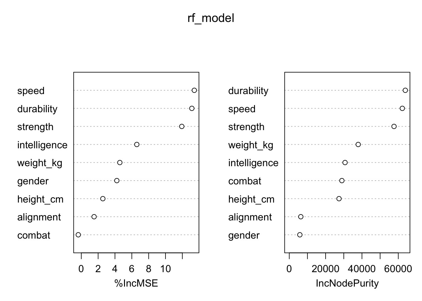
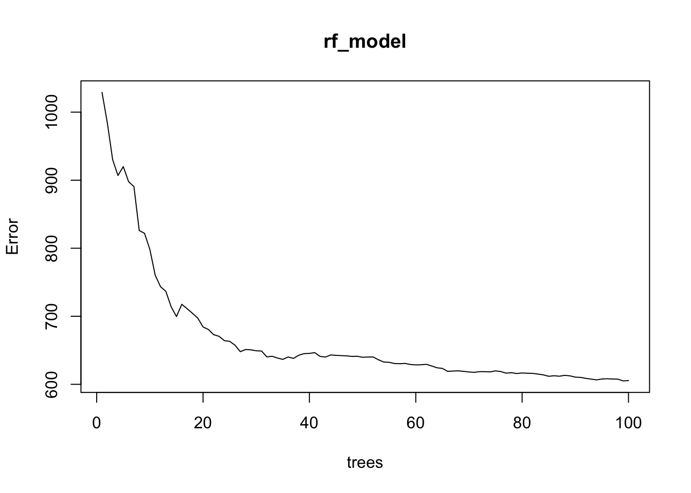
To further verify the importance of selected predictors, a random forest model was trained. We choose to build 100 decision trees and 3 random predictor variables are selected and considered at every split.
##
## Call:
##  randomForest(formula = power ~ combat + strength + speed + durability +      intelligence + height_cm + weight_kg + gender + alignment,      data = superheros_clean1, mtry = 3, ntree = 100, importance = TRUE)
##                Type of random forest: regression
##                      Number of trees: 100
## No. of variables tried at each split: 3
##
##           Mean of squared residuals: 605.4973
##                     % Var explained: 27.19
importance <- importance(rf_model)
varImpPlot(rf_model)
plot(rf_model) From the variable importance plot, we found that speed, durability,
strength, and intelligence are the most important variables for
improving the model’s predictive performance and better fit as they have
a larger %IncMSE and increase in Node Purity, which is consistent with
our model. Therefore, intelligence, Strength, Speed, Durability was
identified as the primary contributors to superheroes’ power.
Final Model
Our final model would be:
lm_modelB <- lm(power ~ intelligence + strength + speed + durability)
Look at Model B:
lm_modelB <- lm(power ~ intelligence + strength + speed + durability, data = superheros_clean1) %>%
  broom::tidy() %>%
  dplyr::select(term, estimate, p.value)

kable(lm_modelB, digits = 4)| term | estimate | p.value |
|---|---|---|
| (Intercept) | 18.5961 | 0.0001 |
| intelligence | 0.2076 | 0.0010 |
| strength | 0.0819 | 0.1012 |
| speed | 0.3402 | 0.0000 |
| durability | 0.2603 | 0.0000 |
Based on the results, intelligence,
Strength, Speed, and Durability
are positively related to power. For one-unit increase in
speed, it causes the largest increase in
power, while one-unit increase in strength
causes the least increase.