Exploratory Data Analysis
library(tidyverse)
library(tidyr)
library(naniar)
library(stringr)
library(janitor)
library(plotly)
library(factoextra)
library(gridExtra)
library(kableExtra)
library(knitr)
library(tableone)
library(fmsb)
Now, we get our neat dataset, superheroes. For this
dataset, we get boxplots for the numerical variables
intelligence, strength, speed,
durability, power, combat,
height_cm, weight_kg which helps us to
understand their distribution. For the categorical variables
publisher, alignment, gender,
eye_color, hair_color, we also analyzed them
accordingly. At the end of this section, we performed a clustering
analysis of all heroes without missing data and categorized them into
three groups: the balanced group, the strength group, and the mediocre
group.
Boxplot and correlation matrix
superheros <- read_csv("data/superheroes.csv")

# Box plot

numeric_vars <- superheros |>
  select(intelligence, strength, speed, durability, power, combat, height_cm, weight_kg)

plots <- lapply(names(numeric_vars), function(var) {
  plot_ly(y = numeric_vars[[var]], type = "box", name = var)
})

boxplot_combined <- subplot(plots, nrows = 3, margin = 0.05)

boxplot_combined
# Correlation Matrix
cor_matrix <- cor(numeric_vars, use = "complete.obs")
cor_heatmap <- plot_ly(
z = cor_matrix,
x = colnames(cor_matrix),
y = colnames(cor_matrix),
type = "heatmap",
colors = colorRampPalette(c("lightblue", "blue", "darkblue"))(100)
) %>%
layout(
title = "Correlation Matrix Heatmap",
xaxis = list(title = "Variables"),
yaxis = list(title = "Variables")
)
cor_heatmapThe first figure shows the distribution of different variables using box plots to visualize the statistical characteristics of multiple superhero attributes.
Intelligence: The median is around 50, with most values
concentrated between 25 and 75, and some low outliers.
Strength: The distribution is fairly even, with almost
no outliers. The median is approximately 50, and the range spans from 0
to 100.
Speed: Most data points are concentrated in the middle
range, with a median slightly above 50, and no obvious outliers.
Durability: The median is around 50, and the overall
distribution is even, ranging from 0 to 100, with almost no
outliers.
Power: The median is close to 50, with a wide range of
values. The overall distribution is relatively symmetric.
Combat: The median is near 50, and the data has a wide
range, with an even distribution and no clear outliers.
Height (cm): Height shows considerable variation, with
some significant outliers, particularly above 500 cm, indicating some
extremely tall superheroes. The median is below 200 cm, with most data
points below 500 cm.
Weight (kg): The median weight is around 100 kg. There
are some very large outliers (over 400 kg), with most values
concentrated below 200 kg.
The second heatmap represents the correlation matrix between several superhero attributes, including intelligence, strength, speed, durability, power, combat, height (in cm), and weight (in kg). The color gradient ranges from light blue to dark blue, where darker shades indicate a stronger positive correlation between two variables. There is a strong correlation between strength and durability (0.65). This suggests that superheroes who are strong also tend to be durable. Height and weight also show a very high correlation (0.69), indicating that taller superheroes tend to be heavier.
Bar chart of publisher
publisher_counts <- superheros |>
  count(publisher) |>
  arrange(desc(n))

publisher_bar <- plot_ly(publisher_counts, x = ~reorder(publisher, -n), y = ~n, type = 'bar', marker = list(color = '#aec7e8')) |>
  layout(title = "Publisher Distribution (Bar Chart - Sorted by Count)",
         xaxis = list(title = "Publisher"),
         yaxis = list(title = "Count"))

publisher_bar
This bar chart represents the distribution of superheroes by publisher, sorted by the number of heroes. The chart shows that Marvel Comics and DC Comics are by far the most dominant publishers, with Marvel having the highest count at 339 heroes, followed by DC Comics with 188 heroes.
Pie Chart of alignment
alignment_counts <- superheros |>
  count(alignment)

alignment_pie <- plot_ly(alignment_counts, labels = ~alignment, values = ~n, type = 'pie',
                        marker = list(colors = c('#98df8a', '#ffbb78', '#9edae5', '#f7b6d2'))) |>
  layout(title = "Alignment Distribution",
         xaxis = list(showgrid = FALSE, zeroline = FALSE, showticklabels = FALSE),
         yaxis = list(showgrid = FALSE, zeroline = FALSE, showticklabels = FALSE))

alignment_pie
This pie chart illustrates the distribution of superhero alignments. The majority of superheroes, about 67.6%, fall under the “Good” category, represented in orange. The second largest segment is the “Bad” alignment, accounting for 28.2%, shown in green. The “Neutral” category, depicted in light blue, represents 3.28% of the characters. Lastly, a tiny slice, labeled as “null” in pink, makes up 0.958% of the characters.
Further analysis for Marvel and DC
marvel_alignment <- superheros |>
  filter(publisher == "Marvel Comics") |>
  count(alignment)

dc_alignment <- superheros |>
  filter(publisher == "Dc Comics") |>
  count(alignment)

# Plot alignment distribution for Marvel Comics
marvel_plot <- plot_ly(marvel_alignment, labels = ~alignment, values = ~n, type = 'pie',
                      marker = list(colors = c('#aec7e8', '#ffbb78', '#98df8a', '#f4cccc'))) |>
  layout(title = "Alignment Distribution - Marvel Comics",
         xaxis = list(showgrid = FALSE, zeroline = FALSE, showticklabels = FALSE),
         yaxis = list(showgrid = FALSE, zeroline = FALSE, showticklabels = FALSE))

# Plot alignment distribution for DC Comics
dc_plot <- plot_ly(dc_alignment, labels = ~alignment, values = ~n, type = 'pie',
                   marker = list(colors = c('#c5b0d5', '#c49c94', '#f9cb9c', '#d9d9d9'))) |>
  layout(title = "Alignment Distribution - DC Comics",
         xaxis = list(showgrid = FALSE, zeroline = FALSE, showticklabels = FALSE),
         yaxis = list(showgrid = FALSE, zeroline = FALSE, showticklabels = FALSE))

marvel_plotdc_plotSince Marvel and DC are the most popular publishers, we checked the distributions of superhero alignments within these two publishers. The two pie chats show the similar distribution as the overall alignments distribution.
Bar Chart for eye and hair color
eye_color_counts <- superheros |>
  count(eye_color)

eye_color_bar <- plot_ly(eye_color_counts,
                         x = ~n,
                         y = ~reorder(eye_color, n),
                         type = 'bar',
                         orientation = 'h',
                         marker = list(color = "#dbdb8d")) |>
  layout(title = "Eye Color Distribution",
         xaxis = list(title = "Count"),
         yaxis = list(title = "Eye Color"))

hair_color_counts <- superheros |>
  count(hair_color)

hair_color_bar <- plot_ly(hair_color_counts,
                          x = ~n,
                          y = ~reorder(hair_color, n),
                          type = 'bar',
                          orientation = 'h',
                          marker = list(color = "#c7c7c7")) |>
  layout(title = "Hair Color Distribution",
         xaxis = list(title = "Count"),
         yaxis = list(title = "Hair Color"))

eye_color_barhair_color_barThis figure contains two bar charts displaying the distribution of superhero eye colors and hair colors. Overall, blue eyes and black hair are the most common features among superheroes.
Demographic Table
superheros1 <- superheros |>
  filter(!is.na(alignment), !is.na(gender))

vars <- c("intelligence", "strength", "speed", "durability", "power", "combat", "height_cm", "weight_kg")

alignment_summary <- CreateTableOne(vars = vars, strata = "alignment", data = superheros1, test = TRUE)

alignment_summary_df <- print(alignment_summary, quote = FALSE, noSpaces = TRUE, printToggle = FALSE)

alignment_summary_df |> as.data.frame() |>
  rename(`p-value` = p) |>
  mutate(test = "F-test") |>
kable()| Bad | Good | Neutral | p-value | test | |
|---|---|---|---|---|---|
| n | 199 | 475 | 22 | F-test | |
| intelligence (mean (SD)) | 68.21 (21.80) | 63.09 (18.66) | 59.77 (17.49) | 0.012 | F-test |
| strength (mean (SD)) | 48.77 (32.95) | 40.89 (32.23) | 54.14 (39.52) | 0.009 | F-test |
| speed (mean (SD)) | 38.86 (23.55) | 39.92 (23.95) | 50.77 (28.77) | 0.092 | F-test |
| durability (mean (SD)) | 63.02 (30.52) | 55.96 (29.12) | 70.55 (31.72) | 0.007 | F-test |
| power (mean (SD)) | 66.48 (29.17) | 62.79 (29.57) | 73.82 (31.33) | 0.129 | F-test |
| combat (mean (SD)) | 62.94 (22.42) | 61.73 (23.27) | 60.59 (23.34) | 0.818 | F-test |
| height_cm (mean (SD)) | 191.61 (26.83) | 184.19 (57.20) | 237.41 (166.78) | 0.001 | F-test |
| weight_kg (mean (SD)) | 140.12 (119.62) | 95.53 (80.17) | 209.50 (223.86) | <0.001 | F-test |
gender_summary <- CreateTableOne(vars = vars, strata = "gender", data = superheros1, test = TRUE)

gender_summary_df <- print(gender_summary, quote = FALSE, noSpaces = TRUE, printToggle = FALSE)

gender_summary_df |> as.data.frame() |>
  rename(`p-value` = p) |>
  mutate(test = "T-test") |>
kable()| Female | Male | p-value | test | |
|---|---|---|---|---|
| n | 200 | 496 | T-test | |
| intelligence (mean (SD)) | 62.46 (15.21) | 65.27 (21.20) | 0.135 | T-test |
| strength (mean (SD)) | 38.36 (32.53) | 45.75 (32.88) | 0.013 | T-test |
| speed (mean (SD)) | 37.03 (21.17) | 41.21 (25.07) | 0.069 | T-test |
| durability (mean (SD)) | 49.82 (28.06) | 62.10 (29.87) | <0.001 | T-test |
| power (mean (SD)) | 61.44 (26.49) | 65.47 (30.66) | 0.153 | T-test |
| combat (mean (SD)) | 60.65 (21.77) | 62.59 (23.45) | 0.376 | T-test |
| height_cm (mean (SD)) | 175.54 (21.88) | 193.35 (67.45) | 0.002 | T-test |
| weight_kg (mean (SD)) | 78.84 (76.98) | 126.88 (110.70) | <0.001 | T-test |
This table summarizes the demographic characteristics of superheroes by alignment (“Bad,” “Good,” “Neutral”) and gender (“Female,” “Male”). The mean and standard deviation are provided for attributes such as intelligence, strength, speed, and others. Significant differences are observed among alignment categories for attributes like intelligence, strength, durability, height, and weight, as indicated by F-test p-values. In the gender comparison, significant differences are found in strength, durability, height, and weight, with males generally showing higher values. These statistical tests highlight notable variations in superhero traits based on alignment and gender.
Clustering analysis
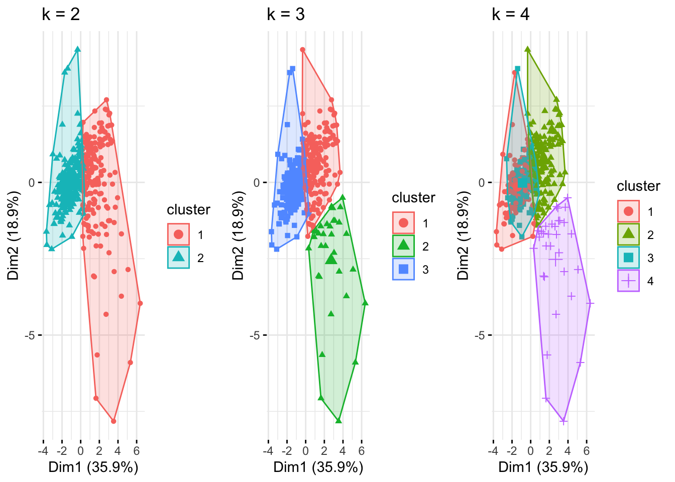
In this section, we use K-means methods to cluster the superheroes
into different groups based on 8 numeric variables:
intelligence, strength, speed,
durability, power, combat,
height_cm, weight_kg. If one superhero has any
missing value of these 8 variables, we exclude this superhero from our
clustering analysis. Finally, 428 superheroes are included in our
analysis.
numeric_vars <- superheros |>
  select(intelligence, strength, speed, durability, power, combat, height_cm, weight_kg)
superheros_clean <- superheros[complete.cases(numeric_vars), ]
numeric_vars_clean <- superheros_clean |>
  select(intelligence, strength, speed, durability, power, combat, height_cm, weight_kg)

numeric_vars_scaled <- scale(numeric_vars_clean)

set.seed(123)

kmeans_result_2 <- kmeans(numeric_vars_scaled, centers = 2, nstart = 25)
plot_2 <- fviz_cluster(kmeans_result_2, data = numeric_vars_scaled,
                       geom = "point",
                       ellipse.type = "convex",
                       ggtheme = theme_minimal()) +
  labs(title = "k = 2")

kmeans_result_3 <- kmeans(numeric_vars_scaled, centers = 3, nstart = 25)
plot_3 <- fviz_cluster(kmeans_result_3, data = numeric_vars_scaled,
                       geom = "point",
                       ellipse.type = "convex",
                       ggtheme = theme_minimal()) +
  labs(title = "k = 3")

kmeans_result_4 <- kmeans(numeric_vars_scaled, centers = 4, nstart = 25)
plot_4 <- fviz_cluster(kmeans_result_4, data = numeric_vars_scaled,
                       geom = "point",
                       ellipse.type = "convex",
                       ggtheme = theme_minimal()) +
  labs(title = "k = 4")

grid.arrange(plot_2, plot_3, plot_4, ncol = 3)
We clustered the 428 superheroes into 2, 3, 4 groups, respectively. We find that dividing superheroes into two categories results in under classification; dividing them into four categories results in reclassification; and dividing them into three categories is the ideal situation.
List of clustering
This is the list of superheroes in each clustering group. Let’s see where your superhero is!
superheros_clean$cluster <- kmeans_result_3$cluster

superheros_clean |>
  group_by(cluster) |>
  summarise(heroes = paste(name, collapse = ", ")) |>
kable()| cluster | heroes |
|---|---|
| 1 | Abe Sapien, Abin Sur, Absorbing Man, Agent Zero, Air-Walker, Alan Scott, Animal Man, Annihilus, Apocalypse, Aqualad, Aquaman, Arachne, Ardina, Ares, Atlas, Atlas, Aurora, Azazel, Battlestar, Beast, Beast Boy, Beta Ray Bill, Big Barda, Bishop, Bizarro, Black Adam, Black Bolt, Black Manta, Blackout, Blob, Booster Gold, Brainiac, Cable, Cannonball, Captain Atom, Captain Britain, Captain Marvel, Captain Marvel, Captain Marvel Ii, Carnage, Century, Cheetah Iii, Citizen Steel, Cloak, Cyborg, Darth Vader, Deadman, Deadpool, Deathstroke, Doc Samson, Doctor Doom, Doctor Fate, Doctor Strange, Doppelganger, Elastigirl, Emma Frost, Etrigan, Evil Deadpool, Evilhawk, Exodus, Firelord, Firestorm, Flash, Flash Ii, Flash Iii, Flash Iv, Franklin Richards, Frenzy, Gamora, Ghost Rider, Gladiator, Goku, Gorilla Grodd, Guy Gardner, Hal Jordan, Hawkgirl, Hela, Hercules, Human Torch, Husk, Hybrid, Hyperion, Iceman, Impulse, Invisible Woman, Iron Fist, Iron Man, Jack Of Hearts, John Stewart, Kang, Klaw, Krypto, Kyle Rayner, Lady Deathstrike, Legion, Lex Luthor, Lizard, Loki, Luke Cage, Mach-Iv, Magneto, Man-Thing, Mantis, Martian Manhunter, Marvel Girl, Maxima, Mephisto, Mera, Metallo, Mimic, Miss Martian, Mister Sinister, Molten Man, Moonstone, Mr Incredible, Namor, Namora, Namorita, Naruto Uzumaki, Northstar, Nova, Nova, Odin, One Punch Man, Phoenix, Plastic Man, Polaris, Power Girl, Predator, Quicksilver, Ray, Red Tornado, Sabretooth, Sandman, Scarlet Spider, Scarlet Witch, Sentry, Shadow King, Shatterstar, She-Thing, Sif, Silver Surfer, Sinestro, Siren, Skaar, Spider-Girl, Spider-Gwen, Spider-Man, Spider-Woman, Starfire, Stargirl, Steel, Steppenwolf, Superboy, Superboy-Prime, Supergirl, Superman, T-1000, Thing, Thor, Thor Girl, Thunderstrike, Thundra, Tiger Shark, Toxin, Toxin, Triton, Ultragirl, Vegeta, Venom, Venom Ii, Vindicator, Vision, War Machine, Warlock, Warpath, Wolverine, Wonder Girl, Wonder Man, Wonder Woman, X-23, X-Man, Zoom |
| 2 | A-Bomb, Abomination, Alien, Amazo, Anti-Venom, Bloodaxe, Colossus, Darkseid, Destroyer, Doomsday, Drax The Destroyer, Hellboy, Hulk, Juggernaut, Killer Croc, Kilowog, Living Brain, Lobo, Machine Man, Modok, Onslaught, Red Hulk, Rhino, Sasquatch, Scorpion, She-Hulk, Solomon Grundy, Spawn, Thanos, Ultron, Venom Iii, Wolfsbane |
| 3 | Adam Strange, Agent Bob, Ajax, Alfred Pennyworth, Angel, Angel Dust, Angel Salvadore, Ant-Man, Ant-Man Ii, Archangel, Arclight, Ariel, Armor, Atom Girl, Atom Ii, Bane, Banshee, Bantam, Batgirl, Batgirl Iv, Batgirl Vi, Batman, Batman, Batman Ii, Big Man, Black Canary, Black Canary, Black Cat, Black Knight Iii, Black Lightning, Black Mamba, Black Panther, Black Widow, Blackwing, Blackwulf, Blade, Bling!, Blink, Blizzard Ii, Boom-Boom, Brainiac 5, Buffy, Bullseye, Bumblebee, Callisto, Captain America, Catwoman, Chamber, Changeling, Cheetah, Cheetah Ii, Clock King, Copycat, Cottonmouth, Crystal, Cyclops, Daredevil, Darkhawk, Darkstar, Dash, Dazzler, Deadshot, Deathlok, Demogoblin, Diamondback, Doctor Octopus, Domino, Electro, Elektra, Elongated Man, Enchantress, Falcon, Feral, Firebird, Firestar, Forge, Franklin Storm, Gambit, Goblin Queen, Gravity, Green Arrow, Green Goblin, Green Goblin Ii, Han Solo, Harley Quinn, Havok, Hawk, Hawkeye, Hawkeye Ii, Heat Wave, Hellcat, Hope Summers, Huntress, Hydro-Man, Indiana Jones, Ink, Jack-Jack, James T. Kirk, Jean Grey, Jennifer Kale, Jessica Jones, John Wraith, Joker, Jolt, Jubilee, Justice, Kingpin, Kraven Ii, Kraven The Hunter, Leader, Light Lass, Lightning Lad, Lightning Lord, Longshot, Luke Skywalker, Man-Wolf, Mandarin, Maverick, Medusa, Meltdown, Metron, Micro Lad, Mister Fantastic, Mister Freeze, Mockingbird, Moon Knight, Morlun, Moses Magnum, Mr Immortal, Ms Marvel Ii, Multiple Man, Mysterio, Mystique, Nebula, Nick Fury, Nightcrawler, Nightwing, Oracle, Paul Blart, Penguin, Phantom Girl, Plantman, Plastique, Poison Ivy, Professor X, Professor Zoom, Psylocke, Punisher, Purple Man, Pyro, Question, Quill, Ra’s Al Ghul, Rambo, Raven, Red Arrow, Red Hood, Red Robin, Red Skull, Rick Flag, Robin, Robin Ii, Robin Iii, Robin V, Rocket Raccoon, Rogue, Ronin, Rorschach, Sage, Scarecrow, Scarlet Spider Ii, Shadow Lass, Shadowcat, Shang-Chi, Shocker, Shriek, Silverclaw, Siryn, Snowbird, Songbird, Space Ghost, Spider-Woman Iii, Spock, Spyke, Star-Lord, Static, Storm, Sunspot, Swarm, Synch, Taskmaster, Tempest, The Comedian, Thunderbird, Tigra, Tinkerer, Toad, Triplicate Girl, Two-Face, Vanisher, Vibe, Violet Parr, Vixen, Vulture, Walrus, Warp, Wasp, Winter Soldier, Wyatt Wingfoot, Yellowjacket, Yellowjacket Ii, Yoda, Zatanna |
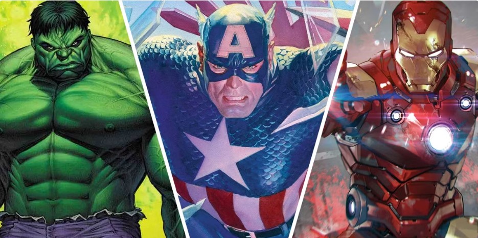
We find that Iron Man, the all-around hero we know, is placed in the first group, strength heroes such as the Hulk are placed in the second group, and mortal heroes such as Captain America are placed in the third group.
Dig into each cluster group
superheros_clean |>
  group_by(cluster) |>
  summarise(
    intelligence_mean = mean(intelligence, na.rm = TRUE),
    intelligence_sd = sd(intelligence, na.rm = TRUE),
    strength_mean = mean(strength, na.rm = TRUE),
    strength_sd = sd(strength, na.rm = TRUE),
    speed_mean = mean(speed, na.rm = TRUE),
    speed_sd = sd(speed, na.rm = TRUE),
    durability_mean = mean(durability, na.rm = TRUE),
    durability_sd = sd(durability, na.rm = TRUE),
    power_mean = mean(power, na.rm = TRUE),
    power_sd = sd(power, na.rm = TRUE),
    combat_mean = mean(combat, na.rm = TRUE),
    combat_sd = sd(combat, na.rm = TRUE),
    height_mean = mean(height_cm, na.rm = TRUE),
    height_sd = sd(height_cm, na.rm = TRUE),
    weight_mean = mean(weight_kg, na.rm = TRUE),
    weight_sd = sd(weight_kg, na.rm = TRUE)
  ) |>
  pivot_longer(-cluster, names_to = c("variable", ".value"), names_sep = "_") |>
  mutate(mean_sd = paste0(round(mean, 2), " (", round(sd, 2), ")")) |>
  select(variable, cluster, mean_sd) |>
  pivot_wider(names_from = cluster, values_from = mean_sd, names_prefix = "cluster") |>
kable()| variable | cluster1 | cluster2 | cluster3 |
|---|---|---|---|
| intelligence | 67.3 (18.18) | 64.16 (22.83) | 62.77 (19.05) |
| strength | 63.93 (28.43) | 76.31 (26.18) | 19.15 (15.04) |
| speed | 54.56 (25.02) | 43.06 (17.41) | 28.38 (14.3) |
| durability | 80.62 (17.83) | 85.72 (19.8) | 38.65 (19.79) |
| power | 81.31 (23.54) | 71.81 (28.23) | 49.62 (25.07) |
| combat | 68.07 (19.15) | 69.47 (20.79) | 59.68 (24.07) |
| height | 184.7 (15.56) | 238.72 (46.7) | 175.79 (15.58) |
| weight | 111.26 (56.52) | 412.97 (180.88) | 74.5 (24.59) |
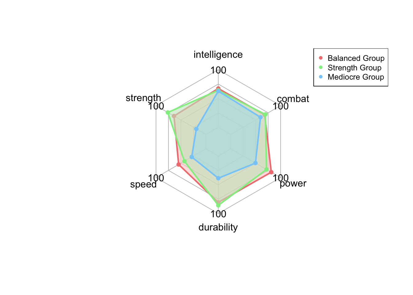
We then calculated the average of the six capability values and two physical values for each clustering to dig into our clustering result, as shown in the table above. We found that the first group of heroes, such as Iron Man, is more versatile (“They are Hexagonal Warriors”). We call the first group “Balanced Group”; The second group of heroes has more strength and staying power, such as Hulk: “Smash! Smash! Smash!” The second group is called the “Strength Group”; The third group of heroes, who are mostly mortals, have significantly lower values than the first two groups, except for intelligence. But they are also the leaders of the team, and their tenacity is infectious to the whole team, as in the case of Captain America. The third group is called the “Mediocre Group”.
Radar Plot!
Below is a visualization of superhero 6 capabilities values in each group from the previous section, using radar charts!
cluster_averages <- superheros_clean |>
  group_by(cluster) |>
  summarise(
    intelligence = mean(intelligence, na.rm = TRUE),
    strength = mean(strength, na.rm = TRUE),
    speed = mean(speed, na.rm = TRUE),
    durability = mean(durability, na.rm = TRUE),
    power = mean(power, na.rm = TRUE),
    combat = mean(combat, na.rm = TRUE)
  )

radar_data <- as.data.frame(cluster_averages)
radar_data <- radar_data[, -1]

radar_data <- rbind(rep(100, 6), rep(0, 6), radar_data)

colors_border <- c('#f08080', '#90ee90', '#87cefa')
colors_in <- c('#ffcccb', '#c6e7c6', '#b0e0e6')

radarchart(radar_data, axistype = 2,
           pcol = colors_border,
           pfcol = adjustcolor(colors_in, alpha.f = 0.6), plwd = 2.5, plty = 1,
           cglcol = "grey", cglty = 1,
           axislabcol = "black")

legend(x = "topright", legend = c('Balanced Group', 'Strength Group', 'Mediocre Group'), pch = 20, col = colors_border, text.col = "black", cex = 0.8, pt.cex = 1)
